Proposal PhD Develope

Indoor positioning

PhD Student: Javad Jafari

Indoor positioning refers to the use of various technologies and methods to determine the location of objects or people inside a building. Unlike outdoor positioning systems, such as GPS, indoor positioning systems (IPS) rely on different technologies due to the lack of satellite signal penetration indoors. Some key technologies and methods used in indoor positioning are as follows:

1. Wi-Fi Positioning Systems (WPS): Utilizes the signal strength of nearby Wi-Fi access points to estimate the position. Often used in large buildings like shopping malls and airports.

2. Bluetooth Low Energy (BLE) Beacons: Small devices that emit signals picked up by smartphones or other devices to calculate the distance to the beacon and triangulate the position.

3. Ultra-Wideband (UWB): Provides high accuracy by using high-frequency radio waves for precise distance measurements. Often used in industrial environments.

4. Infrared (IR) and Visible Light Communication (VLC): Uses light signals to determine location, suitable for environments where radio signals might interfere with other equipment.

5. Radio Frequency Identification (RFID): Uses electromagnetic fields to identify and track tags attached to objects. Useful for asset tracking and inventory management.

6. Magnetic Positioning: Leverages the natural magnetic field variations inside buildings to determine location. Useful in environments where other signals might be obstructed.

7. Inertial Measurement Units (IMU): Combine accelerometers, gyroscopes, and magnetometers to track movement and estimate the position based on movement patterns. Often used in conjunction with other technologies.

8. Vision-based Systems: Use cameras and computer vision algorithms to identify and track the location based on visual cues in the environment.

9. Hybrid Systems: Combine multiple technologies to improve accuracy and reliability. For example, combining Wi-Fi with IMU and BLE beacons.

Indoor positioning systems have a wide range of applications, including:

• Navigation and Wayfinding: Helping people find their way in complex buildings like hospitals, malls, and airports.

• Asset Tracking: Keeping track of valuable equipment and assets in large facilities.

• Retail Analytics: Understanding customer behavior and optimizing store layouts.

• Emergency Response: Locating people in need of assistance during emergencies.

• Smart Buildings: Enhancing building automation and improving energy efficiency.

Unmanifolding

Problem Statement

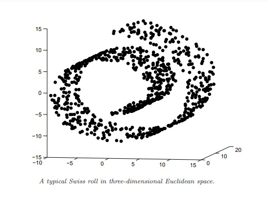
Given a dataset \( \{(\mathbf{x}_i, y_i)\}_{i=1}^N \) where \( \mathbf{x}_i \in \mathbb{R}^d \) and \( y_i \in \mathbb{R} \), the goal is to predict \( y \) from \( \mathbf{x} \). If the data lies on a non-linear manifold \( \mathcal{M} \) in the input space, directly applying regression can lead to suboptimal results because models may cannot capture the non-linear relationships such as swiss roll.

Manifold Representation

A non-linear manifold \( \mathcal{M} \) can be represented as a smooth, continuous surface embedded in a higher-dimensional space \( \mathbb{R}^d \). Mathematically, a point on the manifold can be described as \( \mathbf{x} = \phi(\mathbf{z}) \), where \( \mathbf{z} \in \mathbb{R}^m \) with \( m < d \) and \( \phi \) is a smooth mapping function.

Unmanifolding Concept

The process of unmanifolding involves transforming the data from the non-linear manifold \( \mathcal{M} \) to a linear space \( \mathcal{Z} \) where linear regression can be effectively applied. This transformation can be expressed as a function \( \psi \) such that: $\( \mathbf{z} = \psi(\mathbf{x}) \)\( where \) \mathbf{z} \in \mathbb{R}^m $ is the transformed feature space.

Mapping to the Manifold: $\( \mathbf{x} = \phi(\mathbf{z}) \)\( where \) \phi $ is the mapping from the lower-dimensional latent space to the high-dimensional observation space.

Inverse Mapping (Unmanifolding): $\( \mathbf{z} = \psi(\mathbf{x}) \)\( where \) \psi $ is the inverse mapping or feature extraction function that projects the data back to the lower-dimensional latent space.

Introducing one way for unmanifolding

Neighborhood Graph

Local geometry of the data can be captured using the neighborhood graph. For each data point \(x_i \in D\), its neighbors \(N_i\) are those within a specified radius \(r_N\). This graph structure encodes topological information about the dataset:

\[ N_i = \{i' \in [n] \mid \|x_{i'} - x_i\| \le r_N\} \]

Local Position Matrices \(M_i\)

These matrices \(M_i\) contain the neighbors of each data point \(x_i\):

\[ M_i = [x_{i'} : i' \in N_i] \in \mathbb{R}^{k_i \times D} \]

This matrice provide the local geometry around each point \(x_i\).

Local Embedding Coordinate Matrices \(\Phi_i\)

The local embedding matrices \(\Phi_i\) map the local neighbors into a lower-dimensional space:

\[ \Phi_i = [\phi(x_{i'}) : i' \in N_i] \in \mathbb{R}^{k_i \times m} \]

Here, \(\phi\) is an embedding function that reduces the dimensionality while preserving the local structure. This step is critical in unmanifolding, as it helps to transform the non-linear manifold into a more linear representation.

4. Kernel Matrix \(K\)

The pairwise similarities between data points stored in the kernel matrix \(K\).

\[\begin{split} K_{i,i'} = \begin{cases} \exp \left(-\frac{\|x_i - x_{i'}\|^2}{2\gamma_N^2}\right) & \text{if } i' \in N_i \\ 0 & \text{otherwise} \end{cases} \end{split}\]

Unmanifolding with Neighborhood Graph and Kernel Matrix

Neighborhood Graph

The neighborhood graph captures the local geometry of the data. For each data point \(x_i \in D\), its neighbors \(N_i\) are defined as those within a specified radius \(r_N\):

\[ N_i = \{i' \in [n] \mid \|x_{i'} - x_i\| \le r_N\} \]

This graph encodes topological information about the dataset, preserving the local structure and relationships between data points.

Local Position Matrices \(M_i\)

The local position matrices \(M_i\) contain the samples of the neighbors of each data point \(x_i\):

\[ M_i = [x_{i'} : i' \in N_i] \in \mathbb{R}^{k_i \times D} \]

These matrices represent the local geometry around each point \(x_i\), effectively capturing the local patch of the manifold.

Local Embedding Coordinate Matrices \(\Phi_i\)

The local embedding matrices \(\Phi_i\) map the local neighbors into a lower-dimensional space:

\[ \Phi_i = [\phi(x_{i'}) : i' \in N_i] \in \mathbb{R}^{k_i \times m} \]

Here, \(\phi\) is an embedding function that reduces the dimensionality while preserving the local structure. This step is critical for unmanifolding, as it transforms the non-linear manifold into a more linear representation.

Kernel Matrix \(K\)

The kernel matrix \(K\) encodes the pairwise similarities between data points:

\[\begin{split} K_{i,i'} = \begin{cases} \exp \left(-\frac{\|x_i - x_{i'}\|^2}{2\gamma_N^2}\right) & \text{if } i' \in N_i \\ 0 & \text{otherwise} \end{cases} \end{split}\]

Here, \(\gamma_N\) is the bandwidth parameter, often related to the neighborhood radius \(r_N\) by \(r_N = c \gamma_N\) with \(c\) being a small constant greater than 1. This relationship ensures that the entries in \(K\) that are zeroed out are small, maintaining the matrix’s sparsity.